This course page was updated until March 2022 when I left Durham University. The materials herein are therefore not necessarily still in date.
Models of performance #
If our goal is to improve the performance of some code we should take a scientific approach. We must first define what we mean by performance. So far, we’ve talked about floating point throughput (GFlops/s) or memory bandwidth (GBytes/s). However, these are really secondary characteristics to the primary metric of performance of a code:
How long do I have to wait until I get the answer?
Therefore, we should not lose sight of the overall target of any performance optimisation study, which is to minimise the time to solution for a given code.
Our goal is then to come up with a hypothesis-driven optimisation cycle. A simple flow diagram is shown below

Simplified flow diagram for deciding on next steps when optimising code
The idea is that we decide that the time to solution is too long, and must therefore optimise the code. We profile the code to determine where it spends all (or most) of its time, and then construct a model that explains that time. With a model in hand, we can make a prediction about the best optimisation to apply.
Note that we might not always be able to optimise code such that it can run any faster. So another goal of using a model is to determine that our code really is running is fast as we might expect.
That is, if we start from a position of “my code is running too slowly for my liking”, we need to determine if that is due to a bad implementation, or just hard cheese.
This allows us to focus our optimisation efforts where they will be most effective.
To do this, we need to construct some models, we’ll see a number of approaches in this course, the first one we’ll consider is the roofline model. This is a simple model for loop heavy code.
Exercise
Go away and read that paper, it’s quite approachable. We’ll discuss it in class.
Roofline model #
The roofline model has a simple view of both hardware and software
Simple view of hardware

Simple view of software
/* Possibly nested loops */
for (i = 0; i < ...; i++)
 /* Complicated code doing
    - N FLOPs causing
    - B bytes of data transfer */
This allows us to characterise the code using a single number, its operational intensity, measured in FLOPs/byte
$$ I_c = \frac{N}{B} $$
To this characterisation of the software, we add two numbers that characterise the hardware
- The peak floating point performance \(P_\text{peak}\) measured in FLOPs/s
- The peak streaming memory bandwidth \(B_\text{peak}\) measured in bytes/s
Our challenge is then to ask what the limit on the performance of a piece of code is. We characterise performance by how fast work can be done, measured in FLOPs/s. The roofline model says that the bottleneck is either due to
- execution of work, limited by \(P_\text{peak}\),
- or the data path \(I_c B_\text{peak}\).
We therefore arrive at a bound on performance
$$ P_\text{max} = \text{min}(P_\text{peak}, I_c B_\text{peak}) $$
This is the simplest possible form of the roofline model. It is an optimistic model, everything happens as fast as it possibly can.
Why “roofline” #
Let’s draw a sketch of the performance limits to understand

Sketch of the performance limits for the roofline model
The achievable performance for any code using this model lies underneath the pitched “roof” (hence roofline). The broad idea is that we characterise the hardware once (peak floating point performance, and peak streaming memory bandwidth) and measure $I_c$ for our code along with its floating point performance. We can then plot the performance on a roofline plot, which will give an idea of which performance optimisations are likely to pay off.
A simple example #
For example, consider three exemplar codes, plotted on a roofline

Exemplar roofline plot
The roofline model suggests that there is not really any room to improve the implementation of “Code A”, it’s a memory bandwidth-limited code and achieving that limit.
“Code B” is also memory bandwidth limited, but is not achieving that limit, so there is potentially some room for optimisation.
Finally “Code C” is limited by floating point throughput, and is not close.
This model therefore suggests that we don’t need to do anything with “Code A”, we should look at ways of improving the memory traffic for “Code B”, and we should look at ways of improving the floating point performance of “Code C”.
One thing you may immediately have spotted is that if we only have a roofline plot to hand, we can’t answer our initial question.
There is no way to know how fast these codes get the answer.
Consequently, we should not use it to judge which of a number of different algorithms for a given problem are best (since we may be led to false conclusions).
This is a general rule with optimisation. We start out with lofty goals of improving runtime, but when we start profiling we look at memory bandwidth and floating point throughput. It’s easy to forget that we’re really wanting to improve runtime.
Determining hardware characteristics #
To figure out the performance limits of any given hardware, we have two options:
- Look up values on a spec sheet
- Perform some measurements
Recall that we need two pieces of information, the memory bandwidth and the floating point throughput.
Memory bandwidth #
To look up the maximum achievable bandwidth on a spec sheet, we need
to know the CPU model, as well as what type of RAM is installed. Let’s
do an example with the chips on Hamilton. To determine the installed
chip on a compute node I execute an interactive batch job and look at
the contents of /proc/cpuinfo, looking for the model name
$ ssh hamilton
$ srun --pty $SHELL
$ cat /proc/cpuinfo | grep "model name" | tail -1
model name	: Intel(R) Xeon(R) CPU E5-2650 v4 @ 2.20GHz
Whenever you run the likwid tools they will also report the CPU you were running on.
Then I go to ark.intel.com and search of
E5-2650, I get two results and pick the one at
2.2GHz
I go down to the memory specifications and see that this chip supports 4-channel DDR memory with a frequency of up to 2.4GHz. To compute the maximum achievable memory bandwidth we have
$$ 4 \times 2.4GHz \times 8Byte = 76.8GByte/s $$
Although the memory system can in theory deliver this, it is not achievable by a single core: we’ll see this when we measure stuff later.
If you want lots of details on this, there are some excellent stackoverflow posts: 1, 2, 3.
There are two issues with this:
- I don’t actually know if Hamilton has DDR2400 RAM chips installed
- This is a “guaranteed not to exceed” limit, in practice, even if we do have the right RAM, it is not typically achieved.
The alternative approach, which nearly everyone uses, is to measure the memory bandwidth using the STREAM benchmark. This is what we will typically do, and exercise 4 does exactly that.
Floating point throughput #
Again, the guaranteed not to exceed peak can be determined from spec sheet frequencies and some knowledge of hardware. To do this, let’s look a little at how a CPU core actually works.
If you want much more details on speed limits of compiled code, Travis Downs has a really nice overview. This is article is also a good introduction to lots of the details of modern CPUs.
A simplified picture of a CPU execution engine is shown below (for the Haswell microarchitecture).
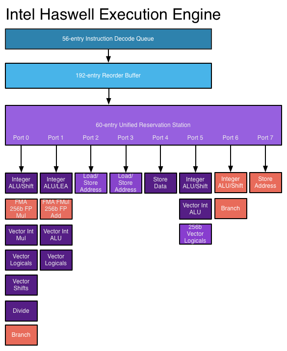
Simplified picture of the Haswell execution engine
The individual assembly instructions in the compiled code are fetched and decoded. They are then scheduled (and possibly reordered) in hardware onto execution ports.
These ports feed the instruction to the execution unit which executes and retires the instruction.
Instructions are issued to the scheduler, but may fail to complete because of data dependencies not being satisfied, or because they were issued in a mis-predicted branch.
An instruction finally completes (leaving the execution pipeline) when it is retired.
Intel chips are 4-way superscalar. That is, they can issue up to 4 μops (or micro-ops) per cycle. However, a port in the execution engine can only execute one μop per cycle. Floating point operations only issue on ports 0 and 1, so our chip can issue at most 2 floating point instructions per cycle.
Fused multiply-add (FMA) instructions (which perform $y ← a + b\times c$) excute on both ports, as do multiplications. However, addition only executes on port 1, and division only on port 0.
If our code basically only executes floating point instructions the best possible case is that we have two SIMD FMA instructions issued per cycle. In this case, the guaranteed not to exceed peak for a single core of the Broadwell chips on Hamilton (which have a peak frequency of 2.9GHz) is
$$ 2.9 \times 2 \times 4 \times 2 = 46.4\text{GFlops/s} $$
We issue 2 FMAs per cycle, each operates on 4 double-precision numbers
(since a double is 64bits and an AVX register is 256bits), so each
instruction does $4\times 2 = 8$ floating point operations.
Conversely, if our code only contains ADD instructions, then the
peak possible performance is only
$$ 2.9 \times 1 \times 4 = 11.6\text{GFlops/s} $$
These calculations are further complicated by frequency scaling. For lots of detail on this, see this excellent article.
To actually hit these limits is remarkably difficult. The FMA instruction has a pipeline latency of 5 on Broadwell chips (4 on Skylake), so to hit the throughput limit, we need 5 in-flight instructions per port, for a total of 10 in-flight instructions. Feeding enough data to these is very difficult. The closest that numerical code typically gets to this in is highly-optimised dense linear algebra libraries.
It is therefore often useful to do two things:
- Measure the achievable floating point peak with LINPACK instead of computing it
- Add multiple floating point limits on our roofline plot, corresponding to different instruction mixes. We will see how we can measure, or estimate, the instruction mix in our code later.
Computing arithmetic intensity #
Now that we’ve characterised our hardware, it’s time to move on to the characterisation of our code. Recall that we need to determine the arithmetic intensity $I_c$: the number of floating point operations performed per byte of data accessed.
There are two approaches we can take here
- Run our code and measure, using performance counters, which we will get to [later](TODO LINK).
- Read the relevant part of the code and count floating point operations and data accesses.
Both approaches have pros and cons, I therefore recommend, if possible to take a blended approach, augmenting measurements with models.
Counting by hand #
Let’s look at a simple example to see how we would go about counting floating point operations and data movement.
Consider the following, very simple, loop:
double *a, *b, *c, *d;
...; /* Allocate memory and initialise */

/* This is the code we've determined to do all the floating point work. */
for (int i = 0; i < N; i++) {
  a[i] = b[i]*c[i] + d[i]*a[i];
}
This code does $N$ iterations of a loop, each iteration performs two multiplications and one addition for a total of $3N$ double precision floating point operations.
Notice how in the simplest case, we don’t care about the type of floating point operation.
Exercise
Given that there are two multiplications and one addition per loop iteration, what is the minimum number of cycles required to execute a single iteration of the loop (ignore any memory load and store operations).
Now let’s try and count the data accesses. Each read counts as one access, each write counts as two (one load, and one store1). We only care about array data so we should ignore any loop variables.
So our loop performs three double precision reads and one double
precision read-write (a[i] appears on both sides) for a total of
$5\times 8$ bytes required per iteration (or $40N$ bytes total).
This seems like we’re now done, in our abstract model, the arithmetic intensity of our code is
$$ I_c = \frac{3N}{40N} = 0.075 \text{flops/byte}. $$
There is one remaining wrinkle. Although it is reasonable to count floating point operations in this manner, the determine the actual data moved we need a model of the cache behaviour of the hardware.
For the loop we just studied, every entry is touched exactly once and then discarded (so we just care about streaming the data). Let’s look at an example where this isn’t the case.
double *a, *b, *c, *d;
...;

for (int i = 0; i < N; i++) {
  for (int j = 0; j < M; j++) {
    a[j] = b[i]*c[i] + d[i]*a[j];
  }
}
In this example, the whole of a is touched for every iteration of
the outer loop. Similarly, each entry of b, c, and d is accessed
j times in the inner loop. A memory-optimal implementation of this
loop would load b[i], c[i], and d[i] into registers for each
iteration of the outer loop and keep all of a in cache for the
duration. However, if the cache is not big enough, we might not
achieve this.
Cache models #
In our analysis, we might not have complete knowledge of the cache sizes, so we can use some simple models. The two extremes are a perfect cache and a pessimal cache.
Perfect cache
This model provides a lower bound on data movement. We assume that each piece of data is moved from main memory exactly once. It therefore counts unique memory accesses.
For the example above, we touch $M$ entries of a with read-write
access (for $8 \times 2 M$ bytes), and we touch $N$ entries each of
b, c, and d with read access (for $8 \times 3 N$ bytes).
So the total data movement for a perfect cache model is $16M + 24N$ bytes.
Pessimal cache
This model provides an upper bound on data movement. We assume that each access misses cache, and so we count the total non-unique memory accesses.
For the example above, there are $MN$ iterations of the loops, so the total data movement for a pessimal cache model is $40 MN$ bytes.
Real code will fall somewhere in between these two extremes: hopefully close to the perfect cache case.
We can also come up with intermediate bounds. In the above example,
suppose that a does not fit in cache, we would expect that the
streaming access to b, c, and d to be fine (because there’s
registere reuse), but we might get no cache hits for a. In this case
we might expect that the total data movement is $8 \times 2 MN +
8\times 3 N = 16 MN + 24 N$ bytes. Since we stream the read arrays
only once, but stream a $N$ times.
Exercise
Suppose $N = 1000$ and $M = 32000$, compute the arithmetic intensities for the above double loop assuming the perfect and pessimal cache models, along with our better intermediate estimate.
The reason to use these models is that they give us bounds on what is achievable by a real code. Measurement of arithmetic intensity only tells us what the code we have does, not what it could do.
Exercise
Go ahead and attempt exercise 4 which looks at producing a roofline model for some different implementations of dense matrix-vector multiplication.
In some cases, they only count as a store, if the compiler can use nontemporal stores ↩︎