This course page was updated until March 2022 when I left Durham University. For future updates, please visit the new version of the course pages.
Supercomputer architecture #
When thinking about the implementation of parallel programming, it is helpful to have at least a high-level idea of what kinds of parallelism are available in the hardware. The different levels of parallelism available in the hardware then map onto (sometimes) different programming models.
Distributed memory parallelism #
Modern supercomputers are all massively parallel, distributed memory, systems. That is, they consist of many processors linked by some network, but do not share a single memory system.
That is, we have a (large) number of computers, often called compute nodes linked by some network.

A small number of compute nodes in a 2D network.
Of course, real supercomputers have many more nodes. For example the present (October 2020) fastest super computer in the world, Fugaku consists of around 400 racks, each containing 384 compute nodes.
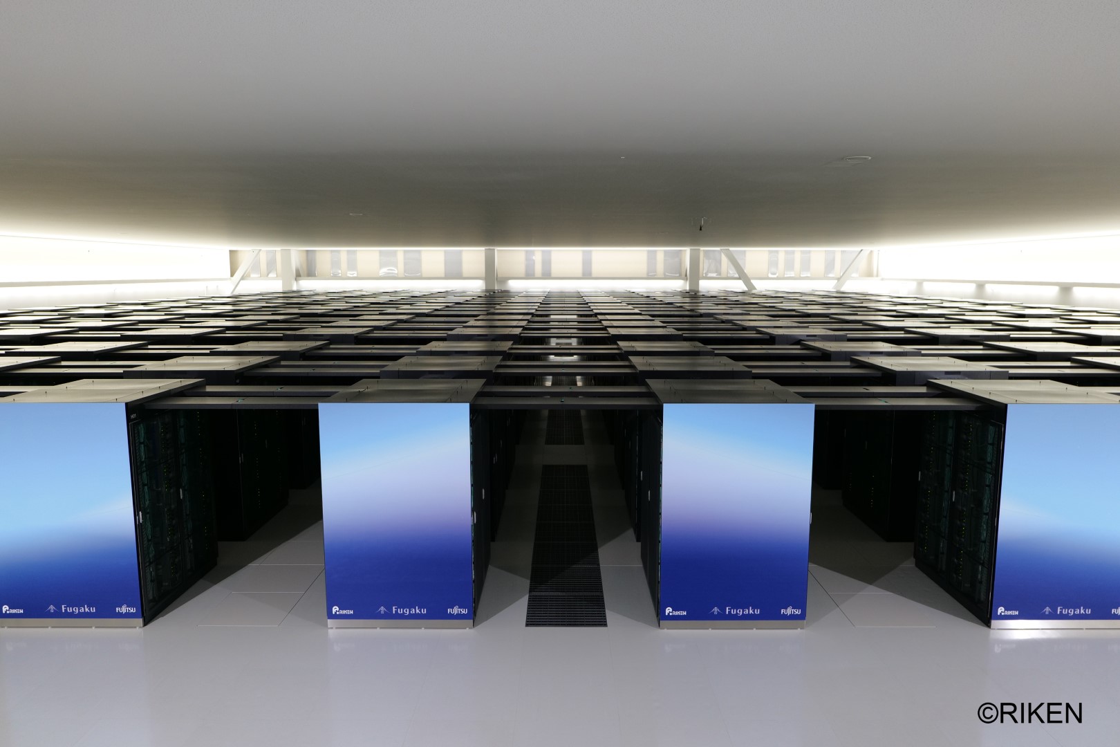
Fugaku machine room.
These different compute nodes do not share a memory space, and so we must use a distributed memory programming model to address the parallelism they offer.
Shared memory parallelism #
Zooming in to a single compute node, we still find multiple levels of parallelism here. As we saw when introducing Moore’s law, despite single-core performance flatlining, transistor counts on chips still do double every 18-24 months.
This exhibits firstly by an increase in the number of CPU cores on any single chip. Rather than having a single CPU attached to some main memory, we might have between four and 64. This is an example of a shared memory system: the different compute units (CPUs) have access to the same piece of shared memory. Sometimes, as sketched in the figure below, there are actually multiple chips all with their attached memory. This is an example of a shared memory compute node with four sockets.

Sketch of a shared memory chip with four sockets.
We can usually program such systems without thinking too hard about the sockets, but we sometimes have to pay attention to where in the memory the data we are computing with resides.
Instruction parallelism #
We’re not quite done in our tour of hardware parallelism. If we now zoom in further to an individual CPU, there is parallelism available here in the instructions that the CPU executes when running our programs. Although there are multiple tricks hardware designers utilise to get the most out of all the transistors on offer, we’ll focus just one, namely vector instructions.
There are other forms of parallelism available on individual CPUs, such as pipelining, superscalar, and out-of-order execution. But these are typically best left to the compiler and hardware, and harder to express in high level code, so we will gloss over them in this course.
Vectorisation is an example of SIMD parallelism. It is the application of the same operation simultaneously to a number of data items. A canonical example of this is operations on arrays of data.
For example, the loop
for (size_t i = 0; i < n; i++)
  a[i] = b[i] + c[i];
might be implemented by \(n\) scalar addition operations, or \(\frac{n}{4}\) vector addition operations (each performing four scalar additions).

Scalar addition, one element at a time

Vector addition, four elements at a time
The rationale for this choice is that it costs about the same power to decode and emit a vector instruction as it does a scalar instruction, but we get four times the throughput! Since we can no longer increase the clock frequency of chips, this is a useful workaround.
Summary #
Parallelism in modern supercomputers spans many scales, from SIMD instruction-level parallelism in which each CPU core might operate on 4-16 floating point values in lockstep, through shared memory parallelism where we might have around 64 CPU cores sharing memory, up to large distributed memory systems where the only limiting factors are the capital budget and ongoing power and cooling costs.
At the present time, there is no one established programming model that covers all of these levels, in this course we will look at how to program for shared memory, and distributed memory parallelism.